gaussians

ctis.scenes.gaussians(inputs, width=None)

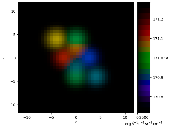
A scene with eight randomly-positioned Gaussian kernels originally prepared by Amy R. Winebarger.

Parameters:

• inputs (DopplerPositionalVectorArray) – The grid of wavelengths and positions on which to evaluate the scene.

• width (None | DopplerPositionalVectorArray) – The standard deviation of the Gaussian kernels. If None (the default), the width will be \(30\,\text{km/s} in the wavelength direction and :math:`1\,\text{arcsec}\) in the spatial directions.

Return type:

FunctionArray[DopplerPositionalVectorArray, ScalarArray]

Examples

Plot this scene for an input grid and standard deviations similar to the one originally tested by Amy R. Winebarger.

import matplotlib.pyplot as plt
import astropy.units as u
import astropy.visualization
import named_arrays as na
import ctis

# Define the spatial plate scale of the instrument
platescale = 0.59 * u.arcsec / u.pix

# Define the grid of positions and velocities on which to evaluate the
# test pattern
inputs = na.DopplerPositionalVectorArray.from_velocity(
    velocity=na.linspace(-500, 500, axis="wavelength", num=21) * u.km / u.s,
    wavelength_rest=171 * u.AA,
    position=na.Cartesian2dVectorLinearSpace(
        start=-20 * platescale * u.pix,
        stop=20 * platescale * u.pix,
        axis=na.Cartesian2dVectorArray("x", "y"),
        num=41,
    ),
)

# Compute the scene of random Gaussians for the
# given input grid and standard deviations
scene = ctis.scenes.gaussians(inputs)

# Plot the result
with astropy.visualization.quantity_support():
    fig, axs = plt.subplots(
        ncols=2,
        gridspec_kw=dict(width_ratios=[.9,.1]),
        constrained_layout=True,
    )
    colorbar = na.plt.rgbmesh(
        C=scene,
        axis_wavelength="wavelength",
        ax=axs[0],
        vmin=0,
        vmax=scene.outputs.max(),
    )
    na.plt.pcolormesh(
        C=colorbar,
        axis_rgb="wavelength",
        ax=axs[1],
    )
    axs[1].yaxis.tick_right()
    axs[1].yaxis.set_label_position("right")