IdealInstrument#

class ctis.instruments.IdealInstrument(area_effective, timedelta_exposure, plate_scale, dispersion, angle, wavelength_ref, position_ref, coordinates_scene, coordinates_sensor, channel, axis_channel, axis_wavelength, axis_scene_xy, axis_sensor_xy, quantum_yield=<Quantity 1. electron / ph>, read_noise=<Quantity 0. electron>, psf=None, axis_psf_xy=('psf_x', 'psf_y'))[source]#

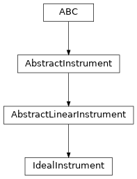
Bases: AbstractLinearInstrument

An idealized CTIS instrument model.

This ideal instrument is characterized by an effective area, exposure time, plate scale and dispersion magnitude/angle.

It has no distortion or vignetting, and it considers only photon shot noise and read noise. It may have a point-spread function, psf.

Attributes

`axis_channel`	The logical axis or axes of this instrument corresponding to the different dispersion magnitudes and angles.
`axis_psf_xy`	The logical axes of `psf` which run along `axis_sensor_xy`.
`axis_scene_xy`	The logical axes of `coordinates_scene` corresponding to changing position coordinate.
`axis_sensor_xy`	The logical axes of `coordinates_sensor` corresponding to changing position coordinate.
`axis_wavelength`	The logical axis of `coordinates_scene` and `coordinates_sensor` that corresponds to changing wavelength coordinate.
`channel`	Human-readable name of each independent CTIS channel.
`coordinates_scene`	A grid of wavelength and position coordinates on the skyplane which will be used to construct the inverted scene.
`coordinates_sensor`	A grid of wavelength and position coordinates on the sensor plane.
`num_channel`	The total number of dispersion magnitudes/angles observed by this instrument.
`psf`	The point-spread function of the instrument on the sensor, or `None` (the default) for none.
`quantum_yield`	The number of electrons generated in the sensor per incident photon, in units equivalent to \(\text{electron} \, \text{photon}^{-1}\).
`read_noise`	The standard deviation of the Gaussian read noise added to each pixel once per readout (after integrating over wavelength), in electrons.
`weights`	The contribution of each voxel on the skyplane to each pixel on the detector.
`weights_transpose`	The contribution of each pixel on the detector to each voxel on the skyplane.
`area_effective`	The effective area of the instrument aperture in units equivalent to \(\text{cm}^2\).
`timedelta_exposure`	The exposure time of the instrument in units equivalent to \(\text{s}\).
`plate_scale`	The spatial scale of the image on the sensor in units equivalent to \(\text{arcsec} \,\text{pix}^-1\)
`dispersion`	The magnitude of the spectral dispersion in units equivalent to \(\text{m \AA} \,\text{pix}^-1\).
`angle`	The angle of the dispersion direction with respect to the scene.
`wavelength_ref`	The reference wavelength at which the center of the FOV lands at `position_ref`
`position_ref`	The position on the sensor where center of the FOV lands at the reference wavelength.

Methods

`__init__`(area_effective, timedelta_exposure, ...)
`backproject`(image[, integrate, unit])	The backward model of this CTIS instrument, which maps photons measured by the sensor to spectral radiance on the skyplane.
`distortion`(coordinates)	A linear mapping between skyplane coordinates and sensor coordinates.
`image`(scene[, integrate, noise, uncertainty])	The forward model of this CTIS instrument, which maps spectral radiance on the skyplane to the electrons measured by the instrument's sensor.

Inheritance Diagram

Parameters:

area_effective (Quantity | AbstractScalar)
timedelta_exposure (Quantity | AbstractScalar)
plate_scale (Quantity | AbstractScalar | Cartesian2dVectorArray)
dispersion (Quantity | AbstractScalar)
angle (Quantity | AbstractScalar)
wavelength_ref (Quantity | AbstractScalar)
position_ref (Quantity | AbstractScalar | Cartesian2dVectorArray)
coordinates_scene (AbstractSpectralPositionalVectorArray)
coordinates_sensor (AbstractSpectralPositionalVectorArray)
channel (str | AbstractScalar)
axis_channel (str | tuple[str, ...])
axis_wavelength (str)
axis_scene_xy (tuple[str, str])
axis_sensor_xy (tuple[str, str])
quantum_yield (Quantity | AbstractScalar)
read_noise (Quantity | AbstractScalar)
psf (None | AbstractScalar)
axis_psf_xy (tuple[str, str])

backproject(image, integrate=True, unit=None)[source]#

The backward model of this CTIS instrument, which maps photons measured by the sensor to spectral radiance on the skyplane.

This is the complementary operation to image(), but it is not an inverse of image(), this method will spread out the photons from each pixel evenly across the voxels in the scene that could have contributed to the measured signal.

Parameters:

image (AbstractScalar | AbstractFunctionArray) – A series of images captured by a CTIS instrument, evaluated on coordinates_sensor, in units of photons.
integrate (bool) – Complement of the integrate keyword of image().
unit (None | UnitBase) – The unit of the backprojected spectral radiance. The forward model, image(), accepts a scene in either photon or energy units, so the backprojection is expressed in whichever the caller requests, converting between photon and energy units using the energy per photon. If None (the default), the radiance is left in the natural units of the backprojection and is not converted.

Return type:

FunctionArray[SpectralPositionalVectorArray, AbstractScalar]

distortion(coordinates)[source]#

A linear mapping between skyplane coordinates and sensor coordinates.

Parameters:: coordinates (SpectralPositionalVectorArray) – Grid of spatial/spectral coordinates on the skyplane.

image(scene, integrate=True, noise=True, uncertainty=False)[source]#

The forward model of this CTIS instrument, which maps spectral radiance on the skyplane to the electrons measured by the instrument’s sensor.

Parameters:

scene (AbstractScalar | AbstractFunctionArray) – The spectral radiance of an observed scene, evaluated on coordinates_scene, in units equivalent to \(\text{erg} \, \text{cm}^{-2} \, \text{sr}^{-1} \, \AA^{-1} \, \text{s}^{-1}\).
integrate (bool) – Whether to integrate along the wavelength axis. A real CTIS instrument integrates along wavelength, but sometimes it’s useful to keep the wavelengths separate for demonstration purposes.
noise (bool) – Whether to include the effect of noise in the final image.
uncertainty (bool) – Whether to attach the standard deviation of the measurement noise to the result, as a NormalUncertainScalarArray. The variance is computed for each wavelength before the integration along the wavelength axis and summed in quadrature, so it is exact even for the integrated image.

Return type:

FunctionArray[SpectralPositionalVectorArray, AbstractScalar]

angle: Quantity | AbstractScalar#: The angle of the dispersion direction with respect to the scene.

area_effective: Quantity | AbstractScalar#: The effective area of the instrument aperture in units equivalent to \(\text{cm}^2\).

axis_channel: str | tuple[str, ...] = <dataclasses._MISSING_TYPE object>#: The logical axis or axes of this instrument corresponding to the different dispersion magnitudes and angles.

axis_psf_xy: tuple[str, str] = ('psf_x', 'psf_y')#: The logical axes of psf which run along axis_sensor_xy.

axis_scene_xy: tuple[str, str] = <dataclasses._MISSING_TYPE object>#: The logical axes of coordinates_scene corresponding to changing position coordinate.

axis_sensor_xy: tuple[str, str] = <dataclasses._MISSING_TYPE object>#: The logical axes of coordinates_sensor corresponding to changing position coordinate.

axis_wavelength: str = <dataclasses._MISSING_TYPE object>#: The logical axis of coordinates_scene and coordinates_sensor that corresponds to changing wavelength coordinate.

channel: str | AbstractScalar = <dataclasses._MISSING_TYPE object>#: Human-readable name of each independent CTIS channel.

coordinates_scene: AbstractSpectralPositionalVectorArray = <dataclasses._MISSING_TYPE object>#

A grid of wavelength and position coordinates on the skyplane which will be used to construct the inverted scene.

Normally the pitch of this grid is chosen to be the average plate scale of the instrument.

coordinates_sensor: AbstractSpectralPositionalVectorArray = <dataclasses._MISSING_TYPE object>#: A grid of wavelength and position coordinates on the sensor plane.

dispersion: Quantity | AbstractScalar#: The magnitude of the spectral dispersion in units equivalent to \(\text{m \AA} \,\text{pix}^-1\).

property num_channel: int#: The total number of dispersion magnitudes/angles observed by this instrument.

plate_scale: Quantity | AbstractScalar | Cartesian2dVectorArray#: The spatial scale of the image on the sensor in units equivalent to \(\text{arcsec} \,\text{pix}^-1\)

position_ref: Quantity | AbstractScalar | Cartesian2dVectorArray#: The position on the sensor where center of the FOV lands at the reference wavelength.

psf: None | AbstractScalar = None#

The point-spread function of the instrument on the sensor, or None (the default) for none.

It is the fraction of the light landing in a pixel which reaches each of the pixels around it, so it is the point-spread function convolved with a pixel twice, once for the pixel the light lands in and once for the pixel it is collected in. Its axes axis_psf_xy run along axis_sensor_xy, and are centered on the element at index \(\lfloor n / 2 \rfloor\). Any other axis is broadcast by name: axis_channel or axis_wavelength give a point-spread function for each channel or wavelength, and axis_sensor_xy one which varies across the sensor.

The point-spread function is folded into weights with named_arrays.regridding.convolve_weights(), so image() blurs the scene by it and backproject(), the transpose, accounts for it too.

quantum_yield: Quantity | AbstractScalar = <Quantity 1. electron / ph>#

The number of electrons generated in the sensor per incident photon, in units equivalent to \(\text{electron} \, \text{photon}^{-1}\).

For this idealized instrument the quantum yield is a constant, so it can be applied after integrating over wavelength.

read_noise: Quantity | AbstractScalar = <Quantity 0. electron>#: The standard deviation of the Gaussian read noise added to each pixel once per readout (after integrating over wavelength), in electrons.

timedelta_exposure: Quantity | AbstractScalar#: The exposure time of the instrument in units equivalent to \(\text{s}\).

wavelength_ref: Quantity | AbstractScalar#: The reference wavelength at which the center of the FOV lands at position_ref

property weights: tuple[AbstractScalar, dict[str, int], dict[str, int]]#: The contribution of each voxel on the skyplane to each pixel on the detector.

property weights_transpose#: The contribution of each pixel on the detector to each voxel on the skyplane.