Invert a Synthetic Scene with MART

In this tutorial, we’ll use the Multiplicative Algebraic Reconstruction Technique (MART) [Gordon et al., 1970] to invert the gaussians() sample scene developed by Amy R. Winebarger. We will use a simple instrument with four projections to image this scene and then use the MART algorithm to reconstruct the original scene.

import IPython.display
import matplotlib.pyplot as plt
import astropy.units as u
import astropy.visualization
import named_arrays as na
import ctis

Start by defining a grid of Doppler velocities on which to reconstruct the scene.

velocity = na.linspace(-500, 500, axis="wavelength", num=21) * u.km / u.s

Define the rest wavelength for converting between velocity and wavelength.

wavelength_rest = 171 * u.AA

Now define a grid of positions on which to reconstruct the scene,

position_scene = na.Cartesian2dVectorLinearSpace(
    start=-10 * u.arcsec,
    stop=10 * u.arcsec,
    axis=na.Cartesian2dVectorArray("scene_x", "scene_y"),
    num=na.Cartesian2dVectorArray(64 + 1, 64 + 1),
)

and a grid of positions on the sensor representing the vertices of each pixel.

position_sensor = na.Cartesian2dVectorArray(
    x=na.arange(0, 128 + 1, axis="sensor_x") * u.pix,
    y=na.arange(0, 64 + 1, axis="sensor_y") * u.pix,
)

Combine the 1D velocity grid and the 2D position grid into a single 3D grid for both the scene and sensor coordinates.

coordinates_scene = na.DopplerPositionalVectorArray.from_velocity(
    velocity=velocity,
    wavelength_rest=wavelength_rest,
    position=position_scene,
)

coordinates_sensor = na.DopplerPositionalVectorArray.from_velocity(
    velocity=velocity,
    wavelength_rest=wavelength_rest,
    position=position_sensor,
)

Create a synthetic scene composed of spatial/spectral 3D Gaussians with various Doppler shifts.

scene = ctis.scenes.gaussians(coordinates_scene)

Add a small background equal to 1 percent of the maximum value of the scene.

scene = scene + scene.max() / 100

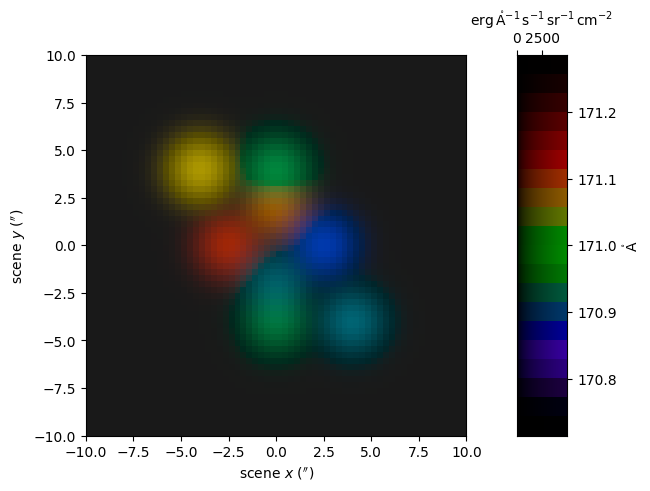
Display the scene as a false-color image.

with astropy.visualization.quantity_support():
    fig, axs = plt.subplots(
        ncols=2,
        gridspec_kw=dict(width_ratios=[.9,.1]),
        constrained_layout=True,
    )
    ax, cax = axs
    colorbar = na.plt.rgbmesh(
        C=scene,
        axis_wavelength="wavelength",
        ax=ax,
        vmin=0,
        vmax=scene.outputs.max(),
    )
    na.plt.pcolormesh(
        C=colorbar,
        axis_rgb="wavelength",
        ax=cax,
    )
    ax.set_aspect("equal")
    ax.set_xlabel(f"scene $x$ ({ax.get_xlabel()})")
    ax.set_ylabel(f"scene $y$ ({ax.get_ylabel()})")
    cax.xaxis.set_ticks_position("top")
    cax.xaxis.set_label_position("top")
    cax.yaxis.tick_right()
    cax.yaxis.set_label_position("right")

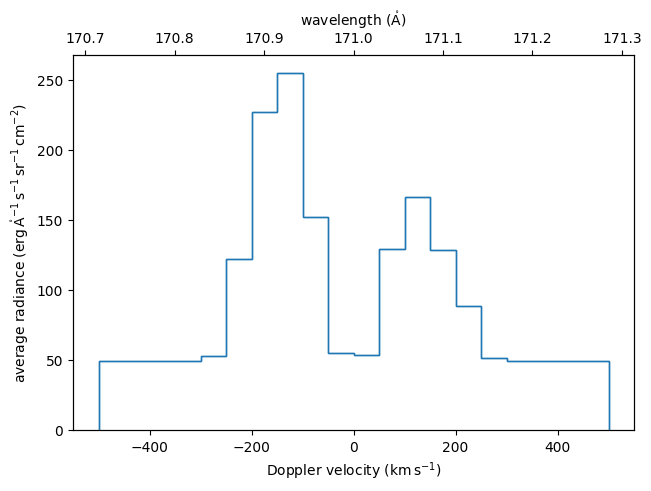
Compute the average spectrum of the scene

spectrum = scene.outputs.mean(("scene_x", "scene_y"))

Plot the average spectrum of the scene.

with astropy.visualization.quantity_support():
    fig, ax = plt.subplots(constrained_layout=True)
    ax2 = ax.twiny()
    na.plt.stairs(
        velocity,
        spectrum,
        ax=ax,
    )
    na.plt.stairs(
        scene.inputs.wavelength,
        spectrum,
        ax=ax2
    )
    ax.set_xlabel(f"Doppler velocity ({ax.get_xlabel()})")
    ax2.set_xlabel(f"wavelength ({ax2.get_xlabel()})")
    ax.set_ylabel(f"average radiance ({ax.get_ylabel()})")

Define the dispersion angles for our instrument. In this case we’ll define four channels, each each separated by \(90^\circ\) degrees.

angle = na.linspace(0, 360, num=4, axis="channel", endpoint=False) * u.deg + 5.64 * u.deg

Define the magnitude of dispersion for our instrument in terms of Doppler velocity and then convert to wavelength units.

dispersion = 10 * u.km / u.s
dispersion = dispersion.to(u.AA, equivalencies=u.doppler_optical(wavelength_rest))
dispersion = (dispersion - wavelength_rest) / u.pix
dispersion.to(u.mAA / u.pix)

$5.703946 \; \mathrm{\frac{m\mathring{A}}{pix}}$

Create an ideal CTIS using the dispersion magnitude and angles.

instrument = ctis.instruments.IdealInstrument(
    area_effective=1 * u.cm ** 2,
    timedelta_exposure=20 * u.s,
    plate_scale=.4 * u.arcsec / u.pix,
    dispersion=dispersion,
    angle=angle,
    wavelength_ref=wavelength_rest,
    position_ref=na.Cartesian2dVectorArray(64, 32) * u.pix,
    coordinates_scene=coordinates_scene,
    coordinates_sensor=coordinates_sensor,
    channel="dispersion angle = " + angle.to_string_array("%03d"),
    axis_channel="channel",
    axis_wavelength="wavelength",
    axis_scene_xy=("scene_x", "scene_y"),
    axis_sensor_xy=("sensor_x", "sensor_y"),
)

Apply the forward model of this instrument to the scene to calculate the observed images.

images = instrument.image(scene)

Display the images as an animation, where each frame represents a different channel / dispersion direction.

with astropy.visualization.quantity_support():
    fig, ax = plt.subplots(
        constrained_layout=True,
        figsize=(9.2, 4),
    )
    norm = plt.Normalize(
        vmin=0,
        vmax=images.outputs.value.ndarray.max(),
    )
    colorizer = plt.Colorizer(
        cmap="gray",
        norm=norm,
    )
    ani = na.plt.pcolormovie(
        instrument.channel,
        images.inputs.position.x,
        images.inputs.position.y,
        C=images.outputs.value,
        axis_time="channel",
        ax=ax,
        kwargs_pcolormesh=dict(
            colorizer=colorizer,
        ),
    )
    plt.colorbar(
        mappable=plt.cm.ScalarMappable(colorizer=colorizer),
        ax=ax,
        label=f"signal ({images.outputs.unit:latex_inline})",
    )
    ax.set_aspect("equal")
    ax.set_xlabel(f"sensor $x$ ({images.inputs.position.x.unit})")
    ax.set_ylabel(f"sensor $y$ ({images.inputs.position.y.unit})")

result = ani.to_jshtml(fps=2)
result = IPython.display.HTML(result)

plt.close(ani._fig)

result

Once Loop Reflect

Initialize the MART inversion algorithm with the instrument model. We’ll also enable saving intermediate results so that we can visualize the behavior of the algorithm.

mart = ctis.inverters.MartInverter(
    instrument=instrument,
    intermediate=True,
)

Invert the images using our instance of MART and the initial guess.

inversion = mart(images)

/home/docs/checkouts/readthedocs.org/user_builds/ctis/envs/latest/lib/python3.11/site-packages/astropy/units/quantity.py:648: RuntimeWarning: invalid value encountered in divide
  result = super().__array_ufunc__(function, method, *arrays, **kwargs)
/home/docs/checkouts/readthedocs.org/user_builds/ctis/envs/latest/lib/python3.11/site-packages/astropy/units/quantity.py:648: RuntimeWarning: divide by zero encountered in divide
  result = super().__array_ufunc__(function, method, *arrays, **kwargs)
/home/docs/checkouts/readthedocs.org/user_builds/ctis/envs/latest/lib/python3.11/site-packages/ctis/inverters/_iterative/_mart/_mart.py:138: UserWarning: Failure: merit increasing.
  warnings.warn(message)

Display the results as a false-color movie, where each frame represents subsequent iterations of the MART algorithm.

with astropy.visualization.quantity_support():
    fig, axs = plt.subplots(
        ncols=3,
        gridspec_kw=dict(width_ratios=[.5, .5, .1]),
        constrained_layout=True,
        figsize=(10, 4.5),
    )
    ax1, ax2, cax = axs
    ax2.set_yticklabels([])
    na.plt.rgbmesh(
        C=scene,
        axis_wavelength="wavelength",
        ax=ax1,
        vmin=0,
        vmax=scene.outputs.max(),
    )
    label = "iteration = " + inversion.iteration.to_string_array("%d") + "\n"
    name = r"$\langle \chi^2 \rangle$"
    label = label + f"{name} = " + inversion.mean_chi_squared.mean(instrument.axis_channel).to_string_array()
    ani, colorbar = na.plt.rgbmovie(
        label,
        scene.inputs.wavelength,
        scene.inputs.position.x,
        scene.inputs.position.y,
        C=inversion.solutions.outputs,
        axis_time=inversion.inverter.axis_iteration,
        axis_wavelength="wavelength",
        ax=ax2,
        vmin=0,
        vmax=scene.outputs.max(),
    )
    na.plt.pcolormesh(
        C=colorbar,
        axis_rgb="wavelength",
        ax=cax,
    )
    ax1.set_title("original")
    ax2.set_title("reconstructed")
    unit_x = scene.inputs.position.x.unit
    unit_y = scene.inputs.position.y.unit
    ax1.set_xlabel(f"scene $x$ ({unit_x:latex_inline})")
    ax2.set_xlabel(f"scene $x$ ({unit_x:latex_inline})")
    ax1.set_ylabel(f"scene $y$ ({unit_y:latex_inline})")
    cax.xaxis.set_ticks_position("top")
    cax.xaxis.set_label_position("top")
    cax.yaxis.tick_right()
    cax.yaxis.set_label_position("right")

result = ani.to_jshtml(fps=20)
result = IPython.display.HTML(result)

plt.close(ani._fig)

result

Once Loop Reflect

Isolate the solution array from the inversion result object.

solution = inversion.solution

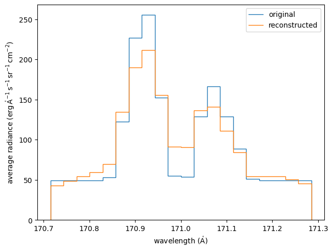
Compute the average spectrum of the reconstructed scene.

spectrum_inverted = solution.outputs.mean(("scene_x", "scene_y"))

Plot the average spectrum of the original scene vs. the average spectrum of the reconstructed scene.

with astropy.visualization.quantity_support():
    fig, ax = plt.subplots(constrained_layout=True)
    na.plt.stairs(
        scene.inputs.wavelength,
        spectrum,
        ax=ax,
        label="original",
    )
    na.plt.stairs(
        scene.inputs.wavelength,
        spectrum_inverted,
        ax=ax,
        label="reconstructed",
    )
    ax.set_xlabel(f"wavelength ({ax.get_xlabel()})")
    ax2.set_xlabel(f"wavelength ({ax2.get_xlabel()})")
    ax.set_ylabel(f"average radiance ({ax.get_ylabel()})")
    ax.legend()

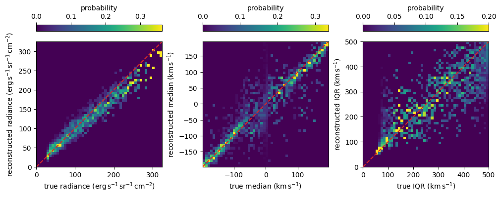
Plot 2D histograms of the true vs. reconstructed value of the total radiance, median (Doppler shift), and interquartile range (Doppler width) for every pixel in the scene.

inversion.plot_moments(scene);

/home/docs/checkouts/readthedocs.org/user_builds/ctis/envs/latest/lib/python3.11/site-packages/named_arrays/_scalars/scalars.py:596: RuntimeWarning: invalid value encountered in divide
  result_ndarray = getattr(function, method)(*inputs_ndarray, **kwargs_ndarray)

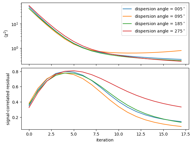
Plot \(\langle \chi^2 \rangle\) and the signal-correlated residual as a function of iteration.

fig, ax = plt.subplots(
    nrows=2,
    sharex=True,
    constrained_layout=True,
)
na.plt.plot(
    inversion.iteration,
    inversion.mean_chi_squared,
    ax=ax[0],
    axis=inversion.inverter.axis_iteration,
    label=instrument.channel,
)
na.plt.plot(
    inversion.iteration,
    inversion.correlation_residual,
    ax=ax[1],
    axis=inversion.inverter.axis_iteration,
    label=instrument.channel,
)
ax[0].set_ylabel(r"$\langle \chi^2 \rangle$")
ax[1].set_xlabel("iteration")
ax[1].set_ylabel("signal-correlated residual")
ax[0].set_yscale("log")
ax[0].legend();