Defining a Simple CTIS Instrument

Here, we construct an idealized example of a CTIS instrument using the IdealInstrument class, an instrument defined by an effective area, plate scale, and dispersion magnitude/angle. This instrument has no point-spread function, distortion, or vignetting, and considers only photon shot noise.

import IPython.display
import numpy as np
import matplotlib.pyplot as plt
import astropy.units as u
import astropy.visualization
import named_arrays as na
import ctis

Start by defining a grid of Doppler velocities.

velocity = na.linspace(-300, 300, axis="wavelength", num=21) * u.km / u.s

Now, define the rest wavelength of a spectral line.

wavelength_rest = 171 * u.AA

Use this rest wavelength to define an astropy.units equivalency between wavelength and Doppler velocity.

AA = dict(unit=u.AA, equivalencies=u.doppler_optical(wavelength_rest))

This equivalency can then be used to convert the grid of Doppler velocities into wavelength units.

wavelength = velocity.to(**AA)

Next, we will define a grid of positions with which to sample the observed scene,

position_scene = na.Cartesian2dVectorLinearSpace(
    start=-10 * u.arcsec,
    stop=10 * u.arcsec,
    axis=na.Cartesian2dVectorArray("scene_x", "scene_y"),
    num=na.Cartesian2dVectorArray(64, 64),
)

and a grid of positions with which to sample the sensor surface.

position_sensor = na.Cartesian2dVectorArray(
    x=na.arange(0, 64, axis="sensor_x") * u.pix,
    y=na.arange(0, 64, axis="sensor_y") * u.pix,
)

Combine the wavelengths and positions into a single spatial-spectral vector for the scene and sensor.

coordinates_scene = na.SpectralPositionalVectorArray(wavelength, position_scene)
coordinates_sensor = na.SpectralPositionalVectorArray(wavelength, position_sensor)

Define the angle of dispersion for each channel of our CTIS instrument. In this case, we’ll define an instrument with 36 dispersion angles to help visualize the behavior of this instrument.

angle = na.linspace(0, 360, num=36, axis="channel", endpoint=False) * u.deg

Define an ideal CTIS instrument, an instrument characterized by an effective area, plate scale, dispersion magnitude/angle, and the coordinates of the scene/sensor.

instrument = ctis.instruments.IdealInstrument(
    area_effective=(0.1 * u.mm**2).to(u.cm**2),
    timedelta_exposure=0.001 * u.s,
    plate_scale=.4 * u.arcsec / u.pix,
    dispersion=((20 * u.km / u.s).to(**AA) - wavelength_rest) / u.pix,
    angle=angle,
    wavelength_ref=wavelength_rest,
    position_ref=32 * u.pix,
    coordinates_scene=coordinates_scene,
    coordinates_sensor=coordinates_sensor,\
    channel="dispersion angle = " + angle.to_string_array("%03d"),
    axis_channel="channel",
    axis_wavelength="wavelength",
    axis_scene_xy=("scene_x", "scene_y"),
    axis_sensor_xy=("sensor_x", "sensor_y"),
)

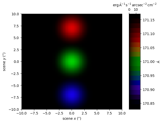
We’ll have our ideal instrument observe a scene of three Gaussians: one at the center of the field of view (FOV) which is at rest, another at the top of the FOV which is redshifted, and a third on the bottom of the FOV which is blueshifted.

center = na.SpectralPositionalVectorArray(
    wavelength=na.ScalarArray([-150, 0, 150] * u.km / u.s, axes="g").to(**AA),
    position=na.Cartesian2dVectorArray(
        x=0 * u.arcsec,
        y=na.ScalarArray([-7, 0, 7] * u.arcsec, axes="g"),
    )
)
width = na.SpectralPositionalVectorArray(
    wavelength=na.ScalarArray(
        ndarray=([25, 25, 25] * u.km / u.s).to(**AA) - wavelength_rest,
        axes="g",
    ),
    position=na.ScalarArray([1, 1, 1] * u.arcsec, axes="g"),
)
amplitude = 1 / np.sqrt(2 * np.pi) / width
radiance = amplitude * np.exp(-np.square(((coordinates_scene - center) / width)) / 2)
radiance = radiance.wavelength * radiance.position.x * radiance.position.y
radiance = radiance * u.erg / u.s / u.cm**2 * 5
radiance = radiance.cell_centers(("wavelength", "scene_x", "scene_y"))
radiance = radiance.sum("g")

scene = na.FunctionArray(
    inputs=coordinates_scene,
    outputs=radiance,
)

Display this scene as a false-color RGB image.

with astropy.visualization.quantity_support():
    fig, axs = plt.subplots(
        ncols=2,
        gridspec_kw=dict(width_ratios=[.9,.1]),
        constrained_layout=True,
    )
    ax, cax = axs
    colorbar = na.plt.rgbmesh(
        C=scene,
        axis_wavelength="wavelength",
        ax=ax,
        vmin=0,
        vmax=scene.outputs.max(),
    )
    na.plt.pcolormesh(
        C=colorbar,
        axis_rgb="wavelength",
        ax=cax,
    )
    ax.set_xlabel(f"scene $x$ ({ax.get_xlabel()})")
    ax.set_ylabel(f"scene $y$ ({ax.get_ylabel()})")
    cax.xaxis.set_ticks_position("top")
    cax.xaxis.set_label_position("top")
    cax.yaxis.tick_right()
    cax.yaxis.set_label_position("right")

Plot the average spectrum of this scene.

with astropy.visualization.quantity_support():
    fig, ax = plt.subplots(constrained_layout=True)
    ax2 = ax.twiny()
    na.plt.stairs(
        velocity,
        scene.outputs.mean(instrument.axis_scene_xy),
        ax=ax,
    )
    na.plt.stairs(
        wavelength,
        scene.outputs.mean(instrument.axis_scene_xy),
        ax=ax2
    )
    ax.set_xlabel(f"Doppler velocity ({ax.get_xlabel()})")
    ax2.set_xlabel(f"wavelength ({ax2.get_xlabel()})")
    ax.set_ylabel(f"average radiance ({ax.get_ylabel()})")

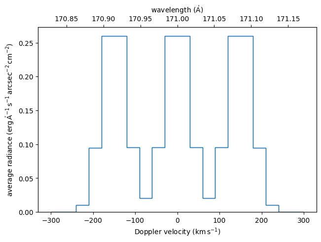
Image the scene onto the sensors using the image() method. In this case, we will not integrate along the wavelength axis to help visualize how different wavelengths are mapped onto the sensor.

image = instrument.image(scene, integrate=False)

Display the images captured by each channel as a false-color animation. Since the dispersion direction is always parallel to the sensor \(x\) axis, the dispersion direction appears fixed as the scene rotates about the center of the FOV.

with astropy.visualization.quantity_support():
    fig, axs = plt.subplots(
        ncols=2,
        gridspec_kw=dict(width_ratios=[.9,.1]),
        constrained_layout=True,
    )
    ax, cax = axs
    ani, colorbar = na.plt.rgbmovie(
        instrument.channel,
        image.inputs.wavelength,
        image.inputs.position.x,
        image.inputs.position.y,
        C=image.outputs,
        axis_time="channel",
        axis_wavelength="wavelength",
        ax=ax,
        vmin=0,
        vmax=image.outputs.max(),
    )
    na.plt.pcolormesh(
        C=colorbar,
        axis_rgb="wavelength",
        ax=cax,
    )
    ax.set_xlabel(f"sensor $x$ ({image.inputs.position.x.unit})")
    ax.set_ylabel(f"sensor $y$ ({image.inputs.position.y.unit})")
    cax.xaxis.set_ticks_position("top")
    cax.xaxis.set_label_position("top")
    cax.yaxis.tick_right()
    cax.yaxis.set_label_position("right")

result = ani.to_jshtml(fps=10)
result = IPython.display.HTML(result)

plt.close(ani._fig)

result

Once Loop Reflect

Now image the scene onto the detectors and integrate along the wavelength axis. The result is a grayscale image that represents what a CTIS instrument actually observes.

image_sum = instrument.image(scene)

Project the measured image back through the scene to find the pixels that could have contributed to the observed signal.

backprojected = instrument.backproject(image_sum)

Display the backprojected images for each channel as an animation .

with astropy.visualization.quantity_support():
    fig, axs = plt.subplots(
        ncols=2,
        gridspec_kw=dict(width_ratios=[.9,.1]),
        constrained_layout=True,
    )
    ax, cax = axs
    ani, colorbar = na.plt.rgbmovie(
        instrument.channel,
        backprojected.inputs.wavelength,
        backprojected.inputs.position.x,
        backprojected.inputs.position.y,
        C=backprojected.outputs,
        axis_time="channel",
        axis_wavelength="wavelength",
        ax=ax,
        vmin=0,
        vmax=backprojected.outputs.max(),
    )
    na.plt.pcolormesh(
        C=colorbar,
        axis_rgb="wavelength",
        ax=cax,
    )
    ax.set_xlabel(f"scene $x$ ({backprojected.inputs.position.x.unit})")
    ax.set_ylabel(f"scene $y$ ({backprojected.inputs.position.y.unit})")
    cax.xaxis.set_ticks_position("top")
    cax.xaxis.set_label_position("top")
    cax.yaxis.tick_right()
    cax.yaxis.set_label_position("right")

result = ani.to_jshtml(fps=10)
result = IPython.display.HTML(result)

plt.close(ani._fig)

result

Once Loop Reflect